About SPOTCLUST
[Please cite]
The ultimate goal of our project is to develop mathematical models for analyzing and merging information in heterogeneous
genotyping and epidemiological databases, and use these models to develop tools for control, understanding, prevention, and
treatment of infectious diseases.
In SPOTCLUST, we focus on Mycobacterium tuberculosis complex (MTC), which includes M. tuberculosis, M.
bovis, M. africanum, M. canetti, and M. microti, because of its great public health importance, data
availability, and our relevant expertise.
Tuberculosis (TB) represents a re-emerging serious health threat worldwide. TB infection continues to grow causing over 2
million deaths each year despite the fact that it is largely curable with proper treatment.
Advances in molecular methods, enriching traditional epidemiology, have contributed significantly to our understanding of the
spread of TB. Differentiating between various patent isolates and using these data to identify epidemiological links are major
molecular epidemiological applications for MTC genotyping.
Our efforts have been concentrated on developing mathematical models for spacer oligonucleotide typing (spoligotyping) data.
Spoligotyping method exploits polymorphism in the direct repeat region of chromosome of the MTC bacteria. This method results in
simple binary pattern for each TB patient and is widely used for MTC strain discrimination.
SPOTCLUST represents a novel approach to advance global studies of MTC genotyping data. It uses mixture models to identify
families within MTC bacteria based on their spoligotyping patterns. SPOTCLUST incorporates biological information on spoligotype
evolution without attempting to derive the full phylogeny of MTC.
We hope that creation of this web site will be followed by generation of comments and suggestions from the scientists with
spoligotyping data of their own. Our goal is to promote active and mutually beneficial collaboration among TB controllers and
biological and computational scientists.
Ideally, to access genetic variability between bacterial strains, we would sequence and then compare their whole genomes. This,
however, is a time-consuming, labor and cost-intensive process, which makes it impractical for TB control. To overcome this
difficulty, only specific genomic loci that bear enough dissimilarity among different strains are used to produce genotypes of
MTC isolates. These molecular genotyping methods exploit the polymorphism in the number and genomic location of repetitive
elements.
In general, to be used as a genetic marker, an element should be locus-specific, polymorphic and easily genotyped. Restriction
fragment length polymorphism (RFLP) analysis with probes derived from the insertion element IS
6110, introduced in 1993
(
van Embden, 1993), is the "gold standard"
method for typing MTC strains (
Mostrom, 2002).
IS
6110 is characterized by
good discriminatory power and high reproducibility. However, it is labor-intensive, requiring culturing of the slow-growing MTC
bacteria for several weeks, and is difficult to standardize between laboratories (
Braden,
2002). Moreover, this method does not
provide sufficient strain discrimination when fewer than five (
van Soolingen, 2001;
Spurgiesz, 2003) or too high number (
Bifani, 2002) of IS
6110-hybridizing bands is present.
Development of PCR-based genotyping methods has greatly improved the typing of MTC strains. PCR-based methods do not require
culturing the bacteria and only small amounts of DNA, which can be obtained directly from the clinical specimen, are sufficient
for analysis. The most widely used PCR-based method is the spoligotyping.
Spoligotyping is based on the polymorphism in the direct repeat (DR) locus of the mycobacterial chromosome (
Kamerbeek, 1997).
The DR locus is one of the most well studied loci of the MTC genome showing considerable strain-to-strain polymorphism (
Fang, 1998). The function
of the DR locus in MTC bacteria is presently unknown (
van Embden, 2000).
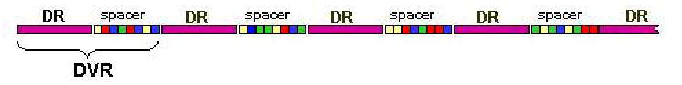
The well-conserved 36-bp direct repeats are interspersed with unique spacer sequences varying from 35 to 41 bp in size. The
order of the spacers was found to be well conserved (
van Embden, 2000). The region comprised the
DR plus the adjacent spacer has been termed the direct variable repeat (DVR) (
Groenen,
1993). Currently, 94 different spacer sequences have been identified of
which 43 are used for MTC strain differentiation (
van Embden, 2000). Clinical isolates of MTC
bacteria can be differentiated by the presence or absence of one or more spacers.
Figure 1:
DR locus (fragment). 43 spacers are used in spoligotyping assay
 |
Each spoligotype can then be conveniently represented as a 43-dimensional binary vector; for example, the most common
spoligotype pattern of
M. tuberculosis Beijing strain is:

. Octal code
designations (
for
M. tuberculosis Beijing) are also widely used (
Dale,
2001).
Spoligotypes are believed to evolve by deletion of a single or multiple contiguous DVRs (
Warren,
2002). Various genetic mechanisms, such as homologous recombination, transposition, DNA replication slippage, or point mutation can
cause the deletion (
Mostrom,
2002;
Warren, 2002). The DR region is one of the hotspots for the IS
6110
integration (
Groenen, 1993;
Legrand, 2001).
Please note that we do not attempt to derive MTC phylogeny based on spoligotyping. Most of the algorithms for phylogenetic trees
are based on the assumption of markers independence. The fact that spoligotypes may evolve by a loss of several adjacent DVRs
(which means that they are dependent on each other) complicates the use of these patterns for deriving MTC phylogeny (
Warren, 2002).
We applied our algorithm to 535 different spoligotype patterns identified among 7166 strains isolated between 1996 and 2004,
primarily from New York State TB patients.
We perform unsupervised classification (clustering) of spoligotyping patterns. Clustering (please do not confuse with finding
clusters of two isolates with matching genotypes) is a process of grouping the objects in the data by some similarity measure.
"Unsupervised" means that we assume no prior knowledge on what family each
spoligotype belongs to. All we start with is our
data, a collection of spoligotypes.
The clustering methods can be divided into two major categories: discriminative (distance-based methods) and generative
(model-based) methods.
Distance-based methods require a metric of pairwise distance between data points. This distance measure is often difficult to
define, especially when the data are complex, for example, biological sequences. Model-based clustering techniques, such as
mixture models, have the advantages that they do not require the distance metric.
The model-based approach is the most appropriate for spoligotypes, because the distance measure between spoligotypes has not
been determined yet. We cannot precisely determine how far is, say,
M. tuberculosis Beijing from
M. bovis, given
their spoligotyping patterns. The belief is that spoligotypes develop by the deletion of spacers, but it is not clear in what
order and how many spacers can be lost simultaneously; therefore, the distance can be probabilistically assessed as a
probability of a "child" spoligotype having been evolved from a "parent"
spoligotype by mostly losing but not gaining
spacers.
We assume that a multivariate Bernoulli mixture model (MBMM) generates the data and that there is a one-to-one correspondence
between mixture model components and spoligotype families. Each model component satisfies the Naïve Bayes assumption.
Naïve Bayes assumption allows treating all the features (in our case, a feature is a presence/absence of a spacer - 1 or 0)
as independent of each other given the class.
Bernoulli distribution has only one parameter,
p, the probability of success (spacer in our case) in a trial with two
possible outcomes. The probability of the absence of a spacer is (1-
p). Thus each position in a spoligotype can be
modeled as a Bernoulli distribution. There are 43 positions; therefore, multivariate Bernoulli distribution (naturally, with 43
parameters, each of which is a probability of a spacer) is used. Finally, we know that there are families within the
spoligotyping data; therefore, some number of different multivariate Bernoulli distributions, each corresponding to a family,
should model the data. Thus we have a mixture of components each corresponding to a distribution.
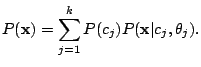
Now let us formalize our probabilistic framework.
Let

be a set of spoligotypes that we want to classify. Each spoligotype is a binary
43-dimensional vector:
. Let

be a mixture model, which consists of

components:
. Each mixture component

is described by parameters

, that are mixing weight of the
component,

, and 43 Bernoulli distributions. The mixing weights satisfy the constrains:
 and and  |
(1) |
The probability of a spoligotype

being generated by
is
 |
(2) |
Thus, to generate a spoligotype, first a mixture component is chosen with a probability
, then its parameters are used
to produce a spoligotype sequence. Let us denote each spacer of
as

(either 0 or 1). Then each mixture
component

has

parameters

, where

is a probability of a spacer being present and

is a
probability of a spacer being absent at a position

of
. The probability of a spoligotype
given component
is:
 |
(3) |
Given the Naïve Bayes assumption, the probability that component
has generated spoligotype
is given as
follows:
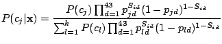 |
(4) |
for

,
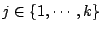
.
The parameters for finite mixture models are often estimated by the maximum likelihood (ML) approach. Expectation-maximization
(EM) is the most commonly used algorithm for finding a local maximum of the likelihood of the observed data.
EM is a class of iterative algorithms for ML estimation useful for a variety of problems with missing data (
Dempster, 1977). On
each iteration of the algorithm , there are two steps, - the expectation (E-) step and the maximization (M-) step. In the
E-step, the expected values of the missing data, given the observed data and the current parameter estimates, are computed so as
to maximize the total log-likelihood. In the M-step, the expected values of the missing data computed in the E-step are used to
re-estimate the parameters and to update the total log-likelihood. The steps are iterated until the difference between current
and subsequent estimates is small.
In the case of our finite mixture model, the missing data is the class (family) labels for each spoligotype. EM iteratively
refines an initial model to better fit the data.
Let  be a collection of n spoligotypes. The number of components in a mixture model with parameters
  is . The
total log-likelihood of , given , is
is . The
total log-likelihood of , given , is
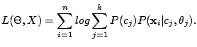 |
(5) |
Iterating between the E- and M-steps results in non-decreasing sequence of values for the total log-likelihood.
The EM algorithm for a mixture of multivariate Bernoulli distributions can be summarized as follows:
Initialization of EM requires a special attention, since the solution of the algorithm is highly dependent upon its starting
points. For MBMM, the initialization includes choosing both the most appropriate parameter values and the number of components
in the mixture.
Model initialization and validation are very important aspects of clustering. We initialized two models - SpolDB3-based and
randomly initialized. As validation criteria, we used the log-likelihood and the stability (or average best match, see Hopcroft, 2004) of the model.
Subsections
To incorporate expert knowledge into our method, we used the published prototypes extracted from a publicly available global
spoligotyping database SpolDB3 ((
Filliol, 2002). These prototypes reflected the expert
defined visual recognition rules
applied to the database.
We extracted seeds (starting parameters for EM) for 32 mixture components (the prototypes for M. africanum and M.
tuberculosis subfamily CAS were combined into seeds for two corresponding components; and the prototype for M. canetti
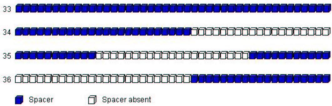
was excluded from the analysis). Based on visual inspection, we supplemented the 32 seeds with four additional prototypes for
spoligotypes that did not match any of the SpolDB3-based prototypes. These four prototypes (ordered for convenience) can
schematically be shown as in Figure 2.
Figure 2:
Four additional prototypes to complement
SpolDB3-based ones
 |
Thus the model, which we called "SpolDB3-based", had 36 components. In other words, the model order was
36. The initial
weights of the components of the mixture were all the same,
 .
.
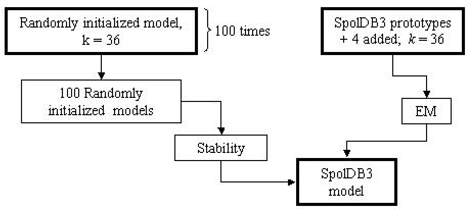
The stability of the clusters produced by a model initialized with SpolDB3-based
prototypes was assessed by comparing the 36
identified families with the families identified by 100 randomly initialized 36-order models (see Figure 3). The stability values for these families gave us an idea of how
reproducible the families were when the model was initialized randomly.
Figure 3:
Schema of analysis of the families identified by SpolDB3-based
model
 |
Another model was initialized randomly. We employed Monte Carlo cross-validation (MCCV) approach (
Smyth, 1996) to find
, the
number of components in the mixture. The schematic representation of MCCV is given in
Figure 4.
Figure 4:
Schema of the MCCV approach used to find the optimal number of clusters
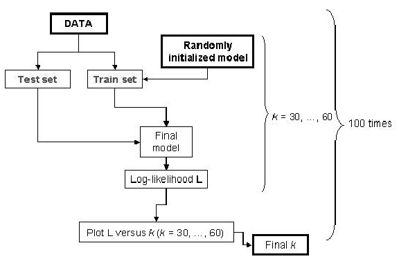 |
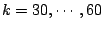
MCCV divides the data randomly 100 (in our case) times into disjoint test and train partitions. The test subset is a fraction
 of the data set. We used = 0.3. For each of the 100 partitions, we vary from
  to
to  , the
values for which are chosen based on our knowledge of the data. We varied from 30 to 60.
, the
values for which are chosen based on our knowledge of the data. We varied from 30 to 60.
First the EM algorithm finds the mixture parameters using the train partition. EM is randomly restarted 10 times and the highest
log-likelihood solution is used as a trained model. EM is initialized using the k-means algorithm that is itself
initialized randomly. At each run out of 10, EM iterates until the total log-likelihood change is less then  or until
the change of the sum of components' weights is less than
or until
the change of the sum of components' weights is less than  . Alternatively, it stops when the number of iterations
achieves 30. For the highest total log-likelihood model, EM is allowed to run 300 additional times or until convergence. Before
starting the 300 iterations, each prototype (where d is a spacer position and j is the mixture component) is modified,
by adding randomness (Juan, 2004):
. Alternatively, it stops when the number of iterations
achieves 30. For the highest total log-likelihood model, EM is allowed to run 300 additional times or until convergence. Before
starting the 300 iterations, each prototype (where d is a spacer position and j is the mixture component) is modified,
by adding randomness (Juan, 2004):
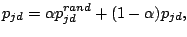 |
(6) |
where

,

,

is a random number, and
measures the ``global randomness''
of
. We used

.
Please find the schema of the random initialization of EM below:
Figure 5:
Schema of random initialization of the EM algorithm
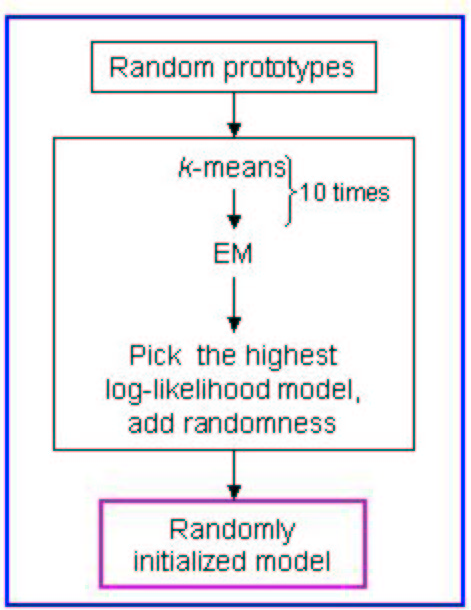 |
Each trained -order model is applied to the test set, and the test data log-likelihood,  is calculated. The procedure is
repeated 100 times and the average (cross-validated) test data log-likelihood,
is calculated. The procedure is
repeated 100 times and the average (cross-validated) test data log-likelihood,
 , is calculated for each .
The plot of
as a function of ( Figure 6) shows what is the most probable for the given
data.
, is calculated for each .
The plot of
as a function of ( Figure 6) shows what is the most probable for the given
data.
Figure 6:
Results of application of MCCV to spoligotyping data: Cross-validated over
100 data partitions test log-likelihoods versus number of clusters,
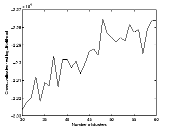 |
We have chosen 48 to be the optimal model order, since this point corresponds to a pick in average test log-likelihoods.
Moreover, after this point, the curve levels off. This indicates that a further increase in the number of parameters will not
improve much the log-likelihood.
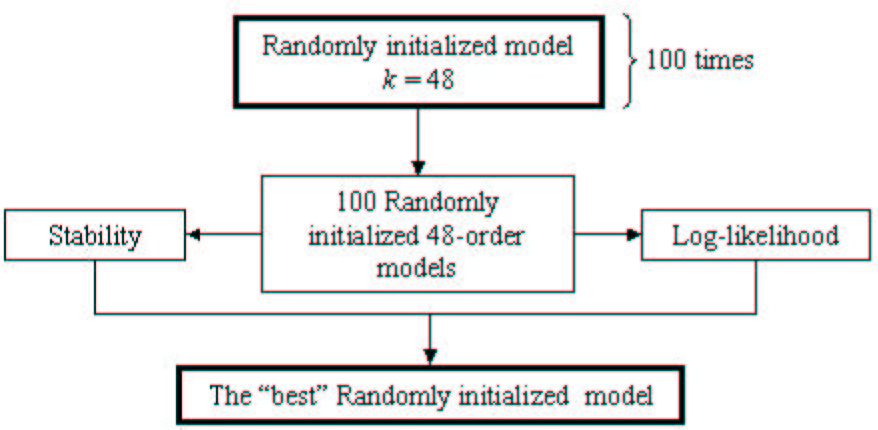
After we had decided on  , we generated, as described above (see Figure 5), 100
randomly initialized mixture
models and calculated the total stabilities (over the resulting families) for each of them relative to the other 99 models. We
chose a final mixture model based on the model stability and the total log-likelihood (see Figure 7).
, we generated, as described above (see Figure 5), 100
randomly initialized mixture
models and calculated the total stabilities (over the resulting families) for each of them relative to the other 99 models. We
chose a final mixture model based on the model stability and the total log-likelihood (see Figure 7).
Figure 7:
Schema of the approach used to find the probabilistically best
model
 |
We call the stability of a cluster (family) of spoligotypes the average best match between the cluster identified by a model and
clusters identified using other models. If we define two clusters and  and treat them as sets, the match (between 0
and
and treat them as sets, the match (between 0
and  ) will be (Hopcroft, 2004):
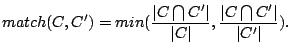 |
(7) |
High match values mean that the sets have many spoligotypes in common and are roughly of the same size.
Figure 8 contains a simple explanation of how the
best match values
were calculated. Here the
best match
values are found for each family identified by Model 1 with respect to Model 2.
Figure 8:
Explanation of calculation of best math values
 |
Since we initialized the 100 models randomly, they each cluster the data into different families. For each cluster in each
model, we calculate the best match with respect to all other models. To calculate the stability of a cluster, we average its
best match values over all of the models, thus obtaining average cluster stability. To find the model stability, we take the
average of stability of the clusters identified by this model.
As we know, it is assumed that DR locus evolves by losing one or multiple contiguous DVRs, and that spacer acquisition is a very
rare event. After we have applied MBMM to our data, we could see that some members of the resulting families did not correspond
to this assumption. This means that in some positions of "children" spoligotypes
(i.e. evolved from a ''parent'' spoligotype,
represented as a prototype for the family) spacers were gained relatively to their ''parent''.
We modified our MBMM by introducing into it Hidden Parent assumption, which helped identifying biologically more relevant
families.
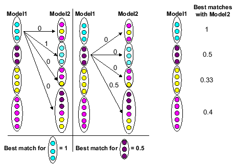
Figure 9:
M. tuberculosis Haarlem2 family
 |
Figure 9 contains SpolDB3 prototype and logos (
Schneider,
1990) of
M. tuberculosis Haarlem2
family identified with and without Hidden Parent. We can see that without Hidden Parent some spacers are occasionally gained,
e.g. spacers 1 - 4 are almost always 0 but are occasionally 1. The model with Hidden Parent fixes this problem.
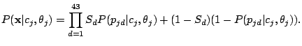
We assume that each spoligotype family has an unobserved Hidden Parent represented by a MBMM, and that the children of the
Parent (the observed strains) may lose a spacer with small probability, but are extremely unlikely to gain one. If we observe
 , then the Hidden Parent of the spoligotype should be generating a 0 with high probability and a 1 with some
non-negligible probability (the child can lose a spacer) at a position . Therefore, the probability of spoligotype x
given mixture component using the Hidden Parent assumption becomes:
, then the Hidden Parent of the spoligotype should be generating a 0 with high probability and a 1 with some
non-negligible probability (the child can lose a spacer) at a position . Therefore, the probability of spoligotype x
given mixture component using the Hidden Parent assumption becomes:
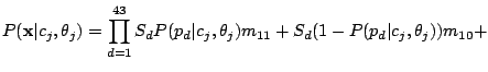 |
|
 |
(8) |
where the probability of losing a spacer is relatively low:
and
,
and the probability of gaining a spacer is extremely low:
,
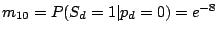
.
The maximum likelihood estimate for (probability of a spacer in position given model component  ), calculated at
the M-step of the EM algorithm, becomes:
), calculated at
the M-step of the EM algorithm, becomes:
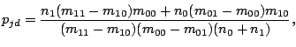 |
(9) |
where
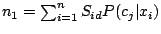
and
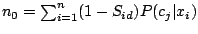
.
We used two MBMMs, SpolDB3-based and randomly initialized; therefore, two sets of families were identified. In this web site,
we give the following information on each of the identified families: a logo (Schneider,
1990) for the spoligotypes from strains forming this family, stability of the family and the data on each spoligotype in the family.
The spoligotype data include NY State number of each spoligotype pattern, number of occurrences of the pattern (i.e., the total number of patients
infected with strains bearing this pattern), probability of the pattern to belong to
the family, the pattern itself in binary
format and octal format, label given by SpolDB3-based model (for families identified by the randomly initialized model), and the
countries of origin of the strains. Families identified by SpolDB3-based model can be viewed in the original order (Filliol, 2002) or sorted by their stabilities.
Please go to families identified by
the SpolDB3-based
Model or to families identified
by the
Randomly Initialized Model.
Please click here if you want
to sumbit your data to SPOTCLUST.
Please send us your
questions, comments, and suggestions.
We would like to emphasize that SPOTCLUST identified spoligotyping families based on the 535 patterns form New York state
patients. Some of the families will be redefined as more data become available. We also plan to expand SPOTCLUST by adding
epidemiological data to it.
1
P.J. Bifani, B. Mathema, N.E. Kurepina, and B.N. Kreiswirth
Global dissemination of the Mycobacterium tuberculosis W-Beijing family strains
Trends Microbiol, 10:45-52, 2002.
2
C.R. Braden, J. T. Crawford, and B.A. Schable
Assessment of Mycobacterium tuberculosis genotyping in a large
laboratory network
Emerg Infect Dis, 8:1210-1215, 2002.
3
J.W. Dale, D. Brittain, A.A. Cataldi, D. Cousins, J.T. Crawford, J. Driscoll et al.
Spacer oligonucleotide typing of bacteria of the Mycobacterium tuberculosis complex: recommendations for standard
nomenclature
Int J Tuber Lung Dis, 5:216-219, 2001.
4
.P. Dempster, N.M. Laird, and D.B. Rubin
Maximum likelihood from incomplete data via the EM algorithm
Journal of the Royal Statistical Society, B(39):1-38, 1977.
5
Z. Fang, N. Morrison, B. Watt, C. Doig, and K.J. Forbes
IS6110 Transposition and Evolutionary Scenario of the Direct Repeat Locus in a Group of Closely Related
Mycobacterium tuberculosis Strains
Int J Bacteriol, 180:2102-2109, 1998.
6
I. Filliol, J.R. Driscoll, D. van Soolingen, B.N. Kreiswirth, K.Kremer, G. Valétudie et al.
Global Distribution of Mycobacterium tuberculosis Spoligotypes
Emerg Infect Dis, 8:1347-1349, 2002.
7
P.M. Groenen, A.E. Bunschoten, D. van Soolingen, and J. D. van Embden
Nature of DNA polymorphism in the direct repeat cluster of Mycobacterium tuberculosis; application for strain
differentiation by a novel typing method
Mol Microbiol, 10:1057-1065, 1993.
8
A. Juan, J. García-Hernández, and E. Vidal
EM initialization for Bernoulli mixture learning
SSPR/SPR, 635-643, 2004.
9
J. Hopcroft, O. Khan, B. Kulis, and B. Selman
Tracking evolving communities in large linked networks
Proc Natl Acad Sci USA, 101:5249-5253, 2004.
10
J. Kamerbeek, L. Schouls, A. Kolk, M. van Agterveld, D. van Soolingen, S. Kuijper et al.
Simultaneous detection and strain differentiation of Mycobacterium tuberculosis for diagnosis and epidemiology
J Clin Microbiol, 35:5907-5914, 1997.
11
E. Legrand, I. Filliol, C. Sola, and N. Rastogi
Use of Spoligotyping To Study the Evolution of the Direct Repeat Locus by IS6110 Transposition in Mycobacterium
tuberculosis
J Clin Microbiol, 39:1595-1599, 2001.
12
P. Mostrom, M. Gordon, C. Sola, M. Ridell, and N. Rastogi
Methods used in the molecular epidemiology of tuberculosis
Clin Microbiol Infect, 8:694-704, 2002.
13
T.D. Schneider and R.M. Stephens
Sequence Logos: A New Way to Display Consensus Sequences
Nucleic Acids Res, 18:6097-6100,1990.
14
P. Smyth
Clustering using Monte Carlo cross-validation
Proceedings of the 2nd International Conference on Knowledge Discovery and Data Mining (KDD-96), Portland, OR, 126-133,
1996.
15
R.S. Spurgiesz, T.N. Quitugua, K.L. Smith, J. Schupp, E.G.Palmer, R.A. Cox, and P. Keim
Molecular Typing of Mycobacterium tuberculosis by Using Nine
Novel Variable-Number Tandem Repeats across the Beijing Family and Low-Copy-Number
IS6110 Isolates
J Clin Microbiol, 41:4224-4230, 2003.
16
J.D.A. van Embden, M.D. Cave, J.T. Crawford and, J. Dale, K.D. Eisenach, B. Gicquel et al.
Strain identification of Mycobacterium tuberculosis by DNA
fingerprinting: recommendations for a standardized methodology
J Clin Microbiol, 31:406-409, 1993.
17
J.D.A. van Embden, T. van Gorkom, K. Kremer, R. Jansen, B.A. van Der Zeijst, and L.M. Schouls
Genetic variation and evolutionary origin of the direct repeat locus of Mycobacterium tuberculosis complex bacteria
J Bacteriol, 9:2393-2401, 2000.
18
D. van Soolingen, D.W. Hermans, P.E. de Haas, D.R. Soll, and J.D.A. van Embden
Occurrence and stability of insertion sequences in Mycobacterium tuberculosis complex strains: evaluation of an insertion
sequence-dependent DNA polymorphism as a tool in the epidemiology of tuberculosis
J Clin Microbiol, 29:2578-2586, 2001.
19
R.M. Warren, E.M. Streicher, S.L. Sampson, G.D. van der Spuy, M. Richardson, D. Nguyen et al.
Microevolution of the Direct Repeat Region of Mycobacterium tuberculosis: Implications for Interpretation of
Spoligotyping Data
J Clin Microbiol, 40:4457-4465, 2002.
This Info section was generated using the
LaTeX2HTML translator Version 2002-2-1 (1.70)
Copyright © 1993, 1994, 1995, 1996,
Nikos Drakos,
Computer Based Learning Unit, University of Leeds.
Copyright © 1997, 1998, 1999,
Ross Moore,
Mathematics Department, Macquarie University, Sydney.
 for
for